Application of Gyro-Theodolite Orientation in Mine Surveying

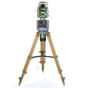
1.Characteristics and working principle of gyro-theodolite

The gyro theodolite uses the axial fixation and precession of the gyro motor when rotating at high speed, and cooperates with the rotation of the earth itself to determine the direction. Within the range of 75° north and south latitude on the earth, it can not be affected by terrain, weather, and geomagnetic field, and can quickly and accurately determine the direction of true north regardless of day or night. Due to its excellent system principles, high precision, and wide range of response capabilities, the gyro-theodolite plays an important role in mine surveying, providing assistance for large-scale measurements such as directional measurements, mine penetration measurements, and contact measurements.

The grade of underground conductors is usually distinguished based on the error in angle measurement. The basic control conductors are 7″ and 15″. When the gyro theodolite starts with a gyro orientation error within the range of plus or minus 7″, the orientation measurement method of attached wire or closed wire terminal is generally used. Sometimes the measurement method of starting edge orientation is also used, which is divided into one well and two wells. Orientation measurement of the downhole starting edge of the well.

Gyro theodolite can effectively reduce the consumption of manpower, material resources and financial resources in the past geometric measurement and orientation work, save time, reduce costs, improve production efficiency and corporate benefits, and because the gyro theodolite can cope with various weather and terrains, It improves the accuracy of directional measurement work under extremely harsh conditions and the measurement accuracy when working on underground planes. The gyro theodolite can carry out precise horizontal directional measurement underground, continuously improve the accuracy with the measurement of control wires, and at the same time check the errors in the measurement of control wires to complete the directional measurement of mines and the penetration of large projects.

2.Application of gyro-theodolite orientation in mine penetration measurement

In mine survey, it is often required that a certain tunnel is connected to another designated tunnel according to the design, which is often referred to as tunnel connection. Usually during penetration operations, multiple excavation tasks are carried out at the same time to improve operation efficiency. At the same time, in order to allow the excavation work to proceed smoothly and ensure that different work teams can accurately carry out the excavation according to the plan, measurements in the predetermined direction must be carried out, which is the through measurement. Through measurement is helpful to ensure the smooth progress of the work, speed up the construction progress, improve the working environment, and ensure that mining and excavation are carried out in the right direction. The penetration measurement usually has the following situations: excavation of two working faces in opposite directions, excavation of two working faces in the same direction, and excavation from one end of the tunnel to the other end. There are three situations of tunnel penetration: tunnel penetration within a mine, mutual penetration between multiple mines, and longitudinal penetration of mine shafts.

The operation steps of gyro theodolite in mine penetration measurement are generally divided into 6 steps:

1) Investigate the hydrogeological conditions of the tunnels to be connected in advance, and select a scientific and systematic measurement method based on the actual situation;

2) Carry out simulation and calculation according to the selected measurement plan;

3) Study the feasibility of the plan based on the calculated results;

4) Determine the measurement plan, determine the geometric characteristics of the through-passage tunnel according to the relevant calculation results, and mark the geometric points of the tunnel on the design drawings and on site;

5) According to the needs of the tunnel connection work, promptly and regularly check various conditions of the tunnel, including the center line, waistline and other geometric elements of the tunnel, regularly check and measure and improve the drawings;

6) After the tunnel penetration work is completed, it is necessary to conduct on-site measurements with a gyro-theodolite in a timely manner, calculate the deviation between the actual penetration results and the measurement, analyze and evaluate the accuracy of the measurement work, and summarize the measurement experience.

The following uses specific engineering examples to introduce the application of gyro-theodolite in mine surveying. A certain mine adopts the freezing method for construction. In order to speed up the construction of the mine, the main tunnel, auxiliary tunnel, and wind shaft tunnel must be constructed through the tunnel, so penetration measurement must be carried out. Conduct a unified inspection of the geometric parameters of the ground control points to determine the geometric characteristics of the measured ground control points; conduct plane and triangular elevation measurements of the air shaft tunnels that pass through the main lanes, and use ground control point arrangements of 5″ and 7″ for the main lanes and auxiliary lanes. The traverse conducts trigonometric elevation measurements. Determine the general parameters of the instrument at a known position on the measuring ground. The gyro theodolite performs a total of 4 measurements, 2 measurements above the well and 2 measurements downhole. The mutual error between all measurement results must be less than 40″. The measurement in the downhole has 1 edge that requires directional measurement. By installing the gyro theodolite on At a fixed position, measure the falling azimuth of the directional edge, and then calculate the geographical azimuth of the directional edge to be measured. Multiple measurements must be made to ensure that the error is less than 25″ to meet the requirements. The azimuth and coordinate angle of each measurement point are already known on the ground. Now we need to calculate the directional edge underground based on the measurement and calculate the coordinate azimuth angle of the corresponding coordinate point. To find the coordinate azimuth angle, you must first find the meridian convergence angle. The geographical azimuth angle is the sum of the coordinate azimuth angle and the meridian convergence angle. The meridian convergence angle is positive or negative. It is positive to the east of the meridian and negative to the west. In the specific measurement, it should be calculated based on the formula of Gaussian coordinates and longitude and latitude of the location where the gyro-theodolite is placed.

3.Application of gyro-theodolite orientation in mine contact measurement

3.1 Casting points

In actual mine measurements, a spring steel wire with a diameter of about 1.5mm is used to drop points from the wellhead downwards. In order to reduce the error during the point throwing process, all fans must be turned off first, stop ventilating the inside of the mine, and use a barrier to Items such as wind boards reduce the impact of wind on the results of point casting. Then put a signal ring down every once in a while to see if the signal ring can fall completely. You can also ask professionals to ride on the equipment to check whether the wire suspension is free and vertical. Place a large bucket filled with stabilizing fluid in the horizontal direction, and the spring After hanging an object of a certain weight on the steel wire, it is sunk into the stabilizing liquid, and then multiple gyro-theodolite are used to perform swing observations in the vertical direction to determine the stabilized position of the spring steel wire.

3.2 Joint testing

When setting the point, it is required to jointly measure the spring steel wire both above and below the mine. Set up a gyro theodolite at the coordinate point on the ground, install a reflector on the wire, and then measure the GK point according to the 5″ wire, still based on the measurement above and below the mine. During the two centering measurements, the measured error must comply with the relevant mine measurement specifications. A gyro theodolite should also be set up underground, and the measurement and spring steel wire joint measurement should be carried out according to the 7″ wire.

4 Factors affecting the directional measurement accuracy of gyro-theodolite

In the measurement work of gyro theodolite, the pendulum orientation accuracy is usually determined by the error in one orientation. Generally speaking, the error in one orientation should be determined during the production process of the gyro theodolite and comply with the specification standards. However, in actual situations, the quality of gyro-theodolite varies and is easily affected by many aspects, including the manufacturer’s manufacturing level, usage environment, daily maintenance, etc. When using reversal point tracking for directional measurement, centering errors, side line mean errors, etc. can easily affect the measurement accuracy.

Summarize

To sum up, in the process of my country’s economic development, for large-scale mine construction projects, errors should be predicted based on the actual conditions of the project, and then directional measurements should be carried out in combination with advanced scientific measurement plans and methods. In mine surveying work, the gyro theodolite is the most widely used measuring instrument. It can adapt to day and night, different latitudes and terrain conditions, ensuring the accuracy of measurement results to the greatest extent. It is of great significance to the development of mine surveying work and mining engineering. Significance. Gyroscopic theodolite from Ericco. For example, ER-GT-02 can achieve more accurate measurements in mine measurements. The orientation accuracy of ER-GT-02 is ≤3.6″ (1σ); it has strong pit interference capability, integrated body design, compact structure, and stable performance; It has functions such as low position locking, automatic zero adjustment and observation.

If you want to learn about or purchase a gyro-theodolite, please contact us.

https://www.ericcointernational.com/info/application-of-gyro-theodolite-orientation-in-mine-surveying.html

Measurement Error and Calibration of FOG IMU

 

1. What causes FOG IMU measurement errors?

Inertial measurement unit is the core component of navigation information and heading attitude reference system, which determines the accuracy and environmental adaptability of the system. Fiber optic gyro is a kind of photoelectric inertial sensor based on Sagnac effect. It has the advantages of high precision, strong resistance to vibration and shock, fast start, etc. It is an ideal angular velocity sensor for rotorcraft, high performance navigation information and heading attitude measurement system. FOG’s adaptability to temperature environment is poor, and the dynamic temperature environment in the working process of rotorcraft is harsh, which leads to the measurement error of FOG IMU. It is necessary to study the precise calibration compensation method of FOG IMU error to improve its environmental adaptability and measurement accuracy.

2. Calibration method
Traditional IMU calibration methods include static multi-position calibration under normal temperature environment, angular rate calibration and hybrid calibration, etc. Among them, static multi-position calibration method can calibrate the error coefficient of IMU acceleration channel with high precision, but due to the small Earth rotation rate, The precision of the small FOG used in the high performance navigation information and heading attitude measurement system of the rotorcraft is similar to the earth rotation rate, resulting in low calibration accuracy of the error coefficient of the angular velocity channel. The error coefficient of FOG IMU angular velocity channel can be accurately calibrated by the traditional simple angular velocity calibration method, but the error coefficient of acceleration channel cannot be accurately calibrated. How to further reduce the calibration workload and improve the calibration accuracy is the key technology to be solved by FOG IMU. In addition, parameters calibrated at room temperature will reduce FOG IMU measurement accuracy if applied at high or low temperatures. Methods such as least squares fitting are often used to compensate the zero-bias or scale-factor temperature errors of inertial devices. Among them, the high-order least squares fitting compensation method can improve the system accuracy, but significantly increase the calculation amount of real-time compensation. The one-time fitting method has a small calculation amount, but it cannot meet the actual compensation accuracy requirements. Therefore, it is another key problem for FOG IMU, a high performance and reliable navigation information and heading attitude measurement system of rotorcraft, to study the compensation method with small amount of computation and high precision.

Based on the FOG IMU integrated error modeling in the high performance navigation information and heading attitude measurement system of rotorcraft, we calibrate and compensate the temperature and dynamic errors of the small low-precision FOG IMU system, and propose a FOG IMU full temperature tripartite positive and negative rate/position calibration method and piecewise linear interpolation compensation method for temperature errors. A tripartite positive and negative speed/one position calibration scheme is designed at each constant temperature point, and piecewise linear interpolation method is used to compensate the zero deviation of angular velocity channel, zero deviation of acceleration channel and scale factor temperature errors. The vehicle-mounted experiments show that the method can improve the system’s environmental adaptability and measurement precision significantly, which lays a foundation for the further development of a small and high-performance fiber optic gyro IMU aircraft navigation information and heading attitude reference system.

3.FOG IMU deterministic error modeling
3.1 Angular velocity channel error model
FOG IMU in rotorcraft, high performance navigation information and heading attitude measurement system consists of three fiber optic gyroscopes and accelerometers, IMU structure and data acquisition and preprocessing module. Three domestic small low-precision 11-FA fiber optic gyroscope sensitive carrier external input angular velocity, three GJ-27 quartz flexible accelerometers sensitive carrier external linear acceleration. FOG is insensitive to g and g2 terms. Considering the installation error, scale factor error and zero bias error of FOG IMU, the angular velocity channel error model of FOG IMU in northeast sky coordinate system is established as

Where, i is the output angular velocity of FOG IMU i axial gyro, and i is the input angular velocity of i axial gyro. i is zero deviation of i axis gyroscope; Ki is the scale factor of i axial gyroscope; Eij is the installation error coefficient of the angular velocity channel, and i and j are collectively referred to as the coordinate axes X, Y and Z.

3.2 Acceleration channel error model
FOG IMU acceleration channel error model is:

Where, ai is the output of FOG IMU i axial addition, ai is the input of i axial addition,  i is zero deviation of i axial addition, Kai is the scale factor of i axial addition, Mij is the installation error coefficient of acceleration channel.

3.3 Full temperature tripartite positive/negative speed/one position calibration
The precision of inertial devices in FOG IMU is mainly related to external environment mechanics and temperature excitation. The operating environment temperature of rotorcraft varies greatly with the different seasons and flight altitudes. Due to the large random dynamic disturbance caused by wind gust and turbulence during successive flights, the influence of different temperatures and dynamic environment on FOG IMU accuracy is mainly studied. The calibration temperature range, temperature point distribution density and calibration dynamic range are set according to the actual working environment and accuracy requirements of the system.
According to the mathematical model of system error, a FOG IMU tripartite positive and negative rate/one position error calibration method is designed based on a temperature-controlled single-axis speed turntable without pointing north and a high-precision hexahedron tool. As shown in Figure 1, the hexahedron tooling is turned three times at each calibrated temperature point to ensure that the X, Y, and Z axes of FOG IMU and the ZT axis of the turntable are reconnected respectively. According to the dynamic environment of the system, set the turntable in each direction to calibrate the positive and negative speed, and ensure that the rotation is above 360° at the speed point.

4. Full temperature piecewise linear interpolation compensation
In order to solve the problem of using FOG IMU in the navigation information and heading attitude measurement system of rotorcraft with high performance and small amount of computation and high precision error compensation, we use the segmented low-order linear interpolation method, dividing the interpolation interval into several cells, and using linear interpolation polynomial on each cell. It can be seen that the FOG IMU angular velocity channel and acceleration channel zero bias, scale factor temperature error piecework linear interpolation compensation algorithm of rotor aircraft operating environment are between -10℃ and 40℃, so the calibration temperature points are set as -10℃, 5℃, 20℃, 30℃ and 40℃ respectively. The FOG IMU is installed in the center of the hexahedron tool, and the X, Y and Z axes of the inertial navigation system are respectively parallel to the datum normal of the hexahedron tool through the high-precision positioning table. Then the hexahedral tooling is fixed horizontally on the plane of the temperature controlled single-axis rate turntable. The three-bit positive and negative speed/one-position calibration as shown in Figure 1 was realized by flipping the hexahedron tooling. Then change the temperature setting value, according to the above method, carry out the calibration experiment at -10℃, 5℃, 20℃, 30 ℃, 40 ℃ in turn.

5. Summary
FOG IMU is the core component of the navigation information and heading attitude reference system of small rotorcraft. ericco’s ER-FIMU-50 and ER-FIMU-70, we can use full-temperature three-way positive and negative rate/one position calibration and PLI compensation method. According to the error characteristics of fiber optic gyro and quartz flexible accelerometer, the FOG IMU error model is established, and the three-bit positive and negative rate/one-position calibration scheme is designed at each constant temperature point. The PLI algorithm is used to compensate the zero bias and scale factor temperature errors of the system in real time, reducing the calibration workload and the calculation amount of the compensation algorithm, and improving the system dynamics, temperature environment adaptability and measurement accuracy.  

Effect of latitude on gyroscopic theodolite

 https://www.ericcointernational.com/application/effect-of-latitude-on-gyroscopic-theodolite.html

Introduce

The gyro-theodolite is a precision directional instrument that is widely used in mining, surveying and mapping and other fields. The pendulum gyro theodolite is currently the most accurate measuring instrument for north finding in engineering applications. It is mainly composed of a gyroscope and a theodolite/total station. This article uses the gyro theodolite for unified description. Its working principle is to realize the true north position measurement by using the component of the earth's rotation angular velocity sensitive to the gyroscope on the gyro sensitive axis, and the angle between the target position and the true north position is determined by the theodolite/total station. Before measuring, the instrument must be leveled to keep the gyro sensitive axis horizontal. Theoretically speaking, the geographical latitude of the instrument when measuring will inevitably have a certain impact on the orientation accuracy and instrument constant stability. The orientation accuracy and instrument constant stability of the gyro-theodolite are key indicators for evaluating the performance of the instrument. The effect of latitude on gyrotheodolite will be introduced in detail below.

Effect of latitude on gyroscopic theodolite

Latitude will have an impact on the north finding of the gyro theodolite. Generally speaking, the gyro theodolite can be used to measure any point within 75° of the north and south geographical latitude. However, for the same instrument, the measurement accuracy will vary when measuring at different latitudes.

1.Relationship between latitude and non-tracking period

The tracking period and the non-tracking period are of great significance to the orientation accuracy of the pendulum gyro theodolite. They are important parameters of the gyro theodolite. They change with the change of latitude. The accuracy of their acquisition or correction can directly affect the performance of the gyro theodolite. Orientation accuracy. The higher the latitude, the larger the non-tracking period.

2.The relationship between latitude and scale coefficient

When the latitude changes, both the tracking period and the non-tracking period change accordingly, and the proportional coefficient is related to the tracking period and the non-tracking period. Its calculation is shown in Equation (1), so the proportional coefficient also changes with the latitude.

(1)

3.The relationship between latitude and pointing moment

The north-pointing moment is the precession moment generated by the horizontal component of the earth's rotation that is sensitive to the gyro system. Its magnitude directly affects the orientation accuracy of the gyro-theodolite, and decreases as the latitude increases. At the equator, the gyro north-pointing moment is the largest. In engineering, the magnitude of the pointing moment is shown in formula (2)

（2）

4.The effect of latitude on orientation accuracy

Theoretically, the orientation accuracy of the gyrotheodolite is the highest at the equator, and the accuracy decreases as the latitude increases. It is generally believed that when the latitude is above 75°, the orientation accuracy of the gyro-theodolite is very low or even impossible. From formula (2) we can know:

When θ=90°, the H-axis points due east (or due west), and the pointing moment is maximum;

When θ=0, the gyro axis is located on the meridian, the north pointing moment is zero, and the gyro is in a steady state;

When Φ = 90°, the gyro-theodolite is located at the earth's poles, the pointing moment is equal to zero, and the gyro-theodolite loses its directional function.

Under the same deflection angle θ, the pointing moment of the gyroscope in low latitudes is larger than that in high latitudes. Theoretically, as long as there is a pointing moment (precession moment), the gyro axis points in the true north direction. However, due to the processing and assembly errors of the gyro, the gyro axis is disturbed or drifts around the meridian plane. To make the gyro seek north normally, it requires a pointing torque to reach a certain level. Therefore, the north seeking range of the gyro should generally be in the north-south geographical direction. Within 75° latitude. Within this latitude range, due to the influence of pointing torque, the north-seeking accuracy of the gyroscope in low-latitude areas is higher than that in high-latitude areas.

Summarize

Through the above analysis, it can be seen that in theory, the higher the latitude, the worse the accuracy of the gyro-theodolite. Latitude affects the pointing moment, instrument constants, proportional coefficients, etc. of the gyro-theodolite, which directly or indirectly affects the measurement accuracy of the instrument. The higher the latitude, the lower the measurement accuracy of the gyro-theodolite. Especially for achieving high-precision gyro north finding, the influence of geographical latitude is one of the factors that needs to be considered. The method of test fitting can be considered to compensate for the latitude influence. As an independently developed inertial navigation company, ERICCO's gyro-theodolite products have relatively high accuracy. For example, the ER-GT-02 ultra-high-precision gyro-theodolite can achieve ultra-high-precision north seeking. Its measurement principle is the integration method and is anti-interference. Features of strong capability and high stability. And ER-GT-02 can also be used in tunnel penetration measurement, subway engineering survey, survey mining, etc.

If you want to learn about or purchase our company's gyro-theodolite, please contact our relevant personnel.

Soft Magnetic Error Compensation Method of Electronic Compass

 

1. Analysis of soft magnetic error of electronic compass

There is another ferromagnetic substance in the working environment of the electronic compass sensor, which, unlike hard ferromagnetic materials, is easily magnetized in a weak magnetic field. When the external magnetic field changes, its induced magnetism will also undergo a related change. The size and direction of the induced magnetic field will also change with the attitude and position of the carrier.
Because of its special properties, this material is called soft iron material. This soft iron material magnetizes itself due to the size of the external magnetic field it receives to produce a magnetic field that resists changes in magnetic flux, which can vary over a wide range. If the magnetic field in the space where the electronic compass sensor is located is known, the magnetic field actually measured by the electronic compass sensor is equal to the superposition of the geomagnetic field and the magnetic field generated by the soft iron interference. The soft iron error is equivalent to a time-varying error superimposed on the output of the electronic compass sensor. Because of the different properties of soft magnetic interference error and hard magnetic interference error, the least square method is no longer applicable when compensating soft magnetic interference error. Soft magnetic interference will lead to the deviation of the measurement Angle of the electronic compass. In an ideal environment, the Angle rotated by the measurement of the electronic compass is controllable, but the existence of soft magnetic interference error will lead to the deviation and uncontrollable Angle of the measurement process of the electronic compass. In the application of navigation system, a small Angle difference will lead to a large route error. The modern electronic compass has strong anti-interference and can suppress most of the Angle deviation, but the compensation of soft magnetic error is still worth studying and discussing.

2. Soft magnetic interference error compensation method
In the actual use of electronic compass, the noise errors caused by soft magnetic interference are mostly random noise errors. At present, there are many algorithms that can be used to compensate random noise and most of them are relatively mature, but considering the characteristics of electronic compass requiring real-time and rapid processing of large amounts of data. Three very mature random noise compensation algorithms, namely Kalman filter, improved Sage adaptive Kalman filter and particle filter, are selected as soft magnetic interference compensation algorithms. These three algorithms are easy to implement and can handle dense data.

2.1 Kalman filter
Kalman filtering algorithm can estimate the linear system with Gaussian white noise, which is the most widely used filtering method at present, and has been well applied in the fields of communication, navigation, guidance and control. The basic idea is that the minimum mean square error criterion is the best estimation criterion, and the future state quantity of the system is estimated by recursion theory, so that the estimated value is as close as possible to the real value.

2.2 Adaptive Kalman filtering
Traditional Kalman filter requires that the mean of dynamic noise and observed noise of the system be zero, and the statistical characteristics are known white noise, but these conditions may not be satisfied in practice, so there are modeling errors. Due to the limitation of objective conditions such as computing tools, the filtering algorithm is easy to produce error accumulation when running on the computer. This results in the loss of positivity or symmetry of error covariance matrix and the instability of numerical calculation.

2.3 Particle filter algorithm
The particle filter algorithm originated from the research of Poor Man's Monte Carlo problem in the 1950s, but the first applied particle filter algorithm was proposed by Gordon et al in 1993. The particle filter is based on the Monte Carlo method, which uses sets of particles to represent probabilities and can be used for any form of state-space model. Particle filter can accurately express the posterior probability distribution based on the observed and controlled quantities, and is a sequential important sampling method. Bayesian inference and importance sampling are the basis of understanding particle filtering.

3. Allan variance simulation experiment 
The Allan analysis of variance is used to simulate the original data of random sequence, the data compensated by Kalman filter algorithm, the data compensated by particle filter algorithm, and the four groups of data compensated by adaptive Kalman filter algorithm. Verify the feasibility of Allan variance analysis algorithm. The Allan standard deviation curve of each data is drawn according to the analysis results. The Allan standard deviation curves of the four groups of data are shown in FIG. 14-17 respectively.

4 Summary
From FIG. 14 to FIG. 17, it can be seen that the Allan variance program of the paper can effectively analyze the experimental data.
Several sets of experimental data show that the program is effective.

After analyzing the data before and after compensation, it can be seen that the quantization noise and zero bias instability noise of the data after compensation by Kalman filter algorithm are reduced by 64% and 66.4% respectively. The quantization noise and zero bias instability noise of the compensated particle filter data are reduced by 70% and 72.1% respectively. The quantization noise and zero bias instability noise of the data compensated by adaptive Kalman filter are reduced by 91.5% and 75.7% respectively. All the algorithms we mentioned can have a better compensation effect for the original data noise.
It can be seen from the compensation effect that compared with traditional Kalman filter and particle filter, adaptive Kalman filter can better remove the noise in the original data, and filter the noise of ER-EC-385, ER-EC-365B and other types of electronic compass. The random data in the simulation experiment is based on the simulation of the noise caused by soft magnetic interference. The simulation results show that the filtering algorithm can compensate the noise of soft magnetic interference.  

IMU denoising method based on wavelet and long short-term memory

 https://www.ericcointernational.com/application/imu-denoising-method-based-on-wavelet-and-long-short-term-memory.html

IMU and GPS fusion algorithm principle

 https://www.ericcointernational.com/application/imu-and-gps-fusion-algorithm-principle.html

How to Improve Accuracy of Tilt Sensors

 

1. Methods to improve the accuracy of tilt sensor

As a very important physical quantity, Angle has a very important position in various fields such as industry, military and aviation, so its measurement is extremely important, and Angle measurement is an important part of metrology science. Tilt sensor is a device to measure the inclination Angle, it is an important link to realize the inclination measurement and automatic control, and its accurate and high-precision measurement becomes the most important thing, so it is necessary to study the algorithm to improve the measurement accuracy.
The research and implementation of the algorithm to improve the accuracy of the tilt sensor are obtained on the basis of practice. The method is based on the arcsine Angle output principle of the tilt sensor. Through repeated data processing and comparison of the old and new error values in the test, the appropriate correlation coefficient is finally obtained, so as to improve the accuracy.

2. Measurement preparation
Measuring the accuracy of biaxial tilt sensor is mainly divided into several steps: making test circuit board, compiling program, building test platform, data acquisition, data analysis and calculation. First of all, it is necessary to make a test circuit board, which is mainly made of dual-axis tilt sensor, single-chip microcomputer, analog-digital converter, MAX232 and other related components.
When the test circuit board is made, it is necessary to use the burner and related software to burn the test program in the single chip microcomputer, as shown in Figure 1. The test circuit board with sensor is fixed on the three-axis turntable, and the circuit board is connected to the computer that collects data, so as to form a complete test device, as shown in Figure 2.

3. Measurement process
After the preparation work is completed, the measurement begins. Along with the rotation of the central axis and the internal axis of the three-axis turntable, the two-axis tilt sensor has the corresponding output value. We collect the data and save it on the computer. After that, the output value is processed, and the output value after data processing is compared with the rotation Angle of the turntable to calculate the accuracy of the sensor. Because the data processing of the central axis and the internal axis is the same, the central axis is introduced here as an example. After many calculations and measurements, the most suitable coefficient is selected to meet the requirements of high precision.
Since the measurement range of the biaxial tilt sensor we selected is between -30℃ and +30℃, here we set the minimum Angle of rotation of the turntable to 5°. Rotation Angle are respectively - 30 °, 25 °, and 20 °, 15 °, and 10 °, 5 °, 0 °, + 5 °, + 10 °, + 15 °, + 20 °, 25 °, 30 ° +, will these values are expressed in Ai. Each time the turntable is rotated, the output value of the sensor is recorded by relevant software, as shown in Figure 3. Among the many output values each time, the minimum and maximum values are recorded, and the data is saved to the computer, as shown in Table 1.

Taking the data at 0° as the benchmark, the output values Ci, Di, Ei and the difference between each output value and the set value Ai Cj, Dj, Ej were calculated using the corresponding formulas

The calculated data table is shown in Table 2.

Curve fitting was performed on Cj, Dj and Ej, as shown in Figure 4.

According to the value 1026 corresponding to 0°, the output value is converted into an Angle, the evaluation test and multiple measurements are carried out. Finally, the optimal values 1028 and 1639 are selected, and the output values Ci, Di, Ei and the difference between each output value and the set value Ai Cj, Dj, Ej are calculated by using the corresponding formulas.

The calculated data table is shown in Table 3. Curve fitting was performed on Cj, Dj and Ej, as shown in Figure 5.

4 Summary
Through measurement and data processing, the requirements for improved accuracy are finally met. As can be seen from Figure 5, the measurement error of the biaxial inclinometer sensor has reached (-0.15~+0.17). To meet higher requirements, the algorithm needs to be further improved.

For our biaxial inclinometer sensors, such as ER-TS-4250VO and ER-TS-4258CU, we can obtain the appropriate correlation coefficient by repeated data processing and comparing the old and new error values in the test through the above algorithm, so as to improve the measurement accuracy of the sensor. 

MEMS IMU error analysis and compensation

https://www.ericcointernational.com/application/mems-imu-error-analysis-and-compensation.html

Electronic Compass Hard Magnetic Error Compensation

 

1. Electronic compass error classification

Electronic compass plays an important role in the navigation application of modern society, because electronic compass is based on the particularity of geomagnetic navigation, digital compass is prone to geomagnetic interference and magnetic material interference in actual use, resulting in measurement errors, according to the source of magnetic interference, can be divided into hard magnetic interference error and soft magnetic interference error. Among them, the hard magnetic interference will cause the zero deviation of the compass measurement value, which will lead to the inaccurate positioning of GPS in the navigation system. It will cause immeasurable impact on activities such as maritime navigation positioning and disaster rescue positioning. Moreover, compensation of hard magnetic interference error is a prerequisite for compensation of soft magnetic interference error. Therefore, before compensation of soft magnetic interference for electronic compass, it is necessary to ensure that the hard magnetic interference error has been compensated, so as to achieve a complete digital compass error compensation process.

2. Hard magnetic error analysis
In the actual working environment of electronic compass sensors, there are inevitably ferromagnetic materials, and one of these ferromagnetic materials is called hard magnetic materials. Because the hard magnetic material has the characteristics of high coercivity, it will be magnetized only in the external magnetic field with sufficient magnetic field strength. Although it is not easy to magnetize hard magnetic materials, the remanent magnetism after it is magnetized will be retained for a long time and is not easy to remove. The magnitude and direction of the magnetic field vector of hard iron in the carrier fixed coordinate system are fixed, and do not change with the course and position of the carrier.

Therefore, the error caused by hard magnetic interference is constant in the short term, which can be considered as a constant additional error output during calibration. At the same time, hard magnetic interference can be used to characterize all time-invariant perturbations of digital compass sensors without losing generality. In the actual measurement and use, the hard magnetic interference will cause the measurement value of the electronic compass to appear obvious deviation, that is, zero drift. In the ideal case of no hard magnetic interference, the electronic compass in the static state, rotating measurement one week, can draw a circle with the center at zero. The hard magnetic error causes the center of the circle to shift, which is called zero drift. Because of the particularity of the hard magnetic error, it can not be avoided and processed by simple physical means, but can only compensate the data collected by the compass to remove the hard magnetic interference error.

3. Hard magnetic interference error compensation method
3.1 Least square method
Generally, the constant error of the sensor is relatively stable, and the corresponding parameters can be obtained by calibration method, and the parameters are introduced into the error calibration equation. To eliminate the constant error of the sensor. Therefore, the error compensation method based on least square method can be adopted. As a kind of mathematical optimization technique, least square method can obtain the best matching function of the optimized object by minimizing the square of the error. Using least squares method can make it easier to obtain unknown data and minimize the sum of squares of error between the obtained data and the actual data. Least squares can also be used for curve fitting. The least square method is the most widely used method in system identification, which can be applied not only to dynamic systems, but also to static systems. It can be used to estimate linear and nonlinear systems as well as offline systems, and the online estimation of systems often uses least square method. In the random environment, when the least square method is used, the observation data does not need to provide its probability and statistics information, but the estimated results have quite good statistical characteristics. The least square method is easy to understand and master, and the recognition algorithm developed based on the least square principle is relatively simple to implement. When other parameter identification methods encounter difficulties, least square method can provide corresponding solutions. The most likely value of unknown model parameters is at the minimum of the sum of repeated error squares between the actual observed value and the calculated value, and the obtained model output can be closest to the output of the actual system, which is the principle of least square.

3.2 Algorithm simulation experiment
The Matlab editor produces a set of standard circle tracks whose center is not at the zero point of the coordinates. The center of the first standard circle is located at the coordinates (2,5) with a radius of 5, as shown in Figure 2. The center of the second standard circle is located at coordinates (114, -304), and the radius is also 5, as shown in Figure 3. It is assumed that the two standard circular trajectories are the actual trajectories measured by the digital compass under hard magnetic interference. Simulation experiments are carried out with the data to verify the feasibility of the algorithm.

The experimental results are shown in FIG. 4 and 5 respectively. After zero deviation compensation, the zero drift of the standard circle is effectively compensated, and the center coordinates of the circle are located at (0,0) after compensation, and the trajectory does not deform. Moreover, good improvement is achieved in both large and small drifts. The simulation results show that the algorithm based on least square method is feasible.

4 Summary
We analyze the source of the hard magnetic error of the electronic compass, select the least square method as the error compensation method according to the error properties, and carry out the program design and simulation experiment based on the least square algorithm to verify the feasibility of the algorithm program. The feasibility and correctness of the algorithm in theory are verified, which lays a foundation for the actual measurement experiment. Ericco's E-compass products such as ER-EC-360A, ER-EC-365A and ER-EC-385CAN have hard magnetic, soft magnetic and inclination compensation functions, so we can use the least square method to compensate its hard magnetic interference error, so that the zero drift can be effectively compensated. 

Research on MEMS IMU error modeling and temperature compensation technology

IMU is a sensor combination used to measure the motion state of an object, mainly composed of a gyroscope and an accelerometer. IMU is usually used in navigation, attitude control, motion tracking and other fields. By measuring the angular velocity and acceleration of an object in three axes, it can calculate the object's attitude, position, speed and other information. The error of MEMS-IMU often requires calibration, which is also important. Then its error can be divided into systematic error and random error. Systematic errors can be eliminated through sensor calibration, while random errors can be understood as the degree of fluctuation and drift of the zero bias. It is usually assumed that the zero bias noise of low-cost MEMS-IMUs obeys a Gaussian distribution. The modeling and compensation of systematic errors and random errors is now an important research direction.

System errors can be eliminated through hardware calibration and software compensation. Hardware calibration usually uses professional calibration equipment to calibrate the IMU, measure the output of each sensor and establish a calibration curve, so that the output can be corrected based on the calibration curve in subsequent use. Software compensation uses algorithms to correct the sensor output, such as using a Kalman filter to perform state estimation and error compensation on the IMU output.

For random errors, temperature compensation technology can be used to reduce them. Since the performance of MEMS sensors is affected by temperature, studying the effect of temperature on sensor output and compensating it is an important technology. Currently, common temperature compensation technologies include neural network compensation, support vector machine compensation, and polynomial fitting compensation. These technologies collect sensor output data at different temperatures, establish a mathematical model of temperature and sensor output, and compensate the sensor output in real time to reduce the impact of temperature on sensor performance.

In addition, in order to further improve the performance of MEMS-IMU, the error transfer function method can also be used to model and compensate the IMU error. This method analyzes the error transfer function of the IMU, establishes a mathematical model of the error transfer function, and compensates the IMU output according to the model. This method can more comprehensively consider the impact of various factors on IMU performance, thereby more accurately estimating the IMU's output and making compensation. This article will talk about MEMS IMU error modeling and MEMS IMU temperature compensation technology.

1.MEMS IMU error modeling

The error modeling of MEMS IMU (Inertial Measurement Unit) mainly focuses on the quantitative description of various error sources in the IMU. These error sources mainly include scale factor error, cross-coupling error, zero bias instability, etc.

The scale factor error and cross-coupling error can be expressed in matrix form and are related to the noise spectrum of the gyroscope and accelerometer. These errors average to zero over time, but any asymmetry or nonlinearity in the scale factor and cross-coupling error will form part of the vibration error and will not cancel each other out over time.

In addition, random errors are also an important source of MEMS IMU errors, mainly including quantization noise, angle (velocity) random walk, bias instability, angular rate (acceleration) random walk and rate ramp, etc. Among them, angle (velocity) random walk and zero-bias instability are the main manifestations of MEMS IMU.

In order to reduce these errors, various compensation methods can be used. For example, system errors are eliminated through hardware calibration and software compensation, and the impact of random errors is reduced through temperature compensation technology. Temperature compensation technology can collect sensor output data at different temperatures, establish a mathematical model of temperature and sensor output, and compensate the sensor output in real time based on the model.

In addition, the error transfer function method can also be used for error modeling of MEMS IMU. By analyzing the error transfer function of the IMU, a mathematical model of the error transfer function is established, and the output of the IMU is compensated based on the model. This method can more comprehensively consider the impact of various factors on IMU performance, thereby more accurately estimating the IMU's output and making compensation.

In general, error modeling of MEMS IMU is a complex process that requires comprehensive consideration of multiple factors and methods. Through in-depth understanding and research of sensor performance, continuous optimization of compensation algorithms and improvement of manufacturing processes, the performance and reliability of MEMS IMU can be improved, providing important technical support for the development and application of navigation, positioning, attitude control and other fields.

2.MEMS IMU temperature compensation technology

The temperature compensation technology of MEMS IMU mainly studies the impact of temperature on sensor performance and takes corresponding methods to reduce this impact. The following are several common temperature compensation methods:

2.1 Hardware Calibration and Compensation: By calibrating the IMU during the manufacturing process, the output of each sensor is measured and a calibration curve is established. In actual use, the output of the IMU is corrected according to the calibration curve to reduce the impact of temperature on sensor performance.

2.2 Establish a mathematical model: By collecting the output data of the sensor at different temperatures, establish a mathematical model of temperature and sensor output. This model is used to compensate the sensor output in real time to reduce the impact of temperature on sensor performance. Common mathematical models include polynomial fitting, linear regression, and neural networks.

2.3 Error transfer function: By analyzing the error transfer function of the IMU, a mathematical model of the error transfer function is established. Compensating the output of the IMU based on this model can more comprehensively consider the impact of various factors on the performance of the IMU, thereby more accurately estimating the output of the IMU and performing compensation.

2.4 Dynamic adjustment: In some cases, the impact of temperature on sensor performance can be reduced by dynamically adjusting the operating parameters of the IMU. For example, by adjusting parameters such as sampling frequency and gain, the performance of the IMU at different temperatures can be made more stable.

In summary, temperature compensation technology for MEMS IMUs requires selecting an appropriate method based on the specific situation. Through in-depth understanding and research of sensor performance, continuous optimization of compensation algorithms and improvement of manufacturing processes, the performance and reliability of MEMS IMU can be improved, providing important technical support for the development and application of navigation, positioning, attitude control and other fields.

Summarize

In general, research on IMU error modeling and temperature compensation technology based on MEMS is an important research direction. By in-depth study of the error sources and characteristics of MEMS-IMU, and using appropriate calibration and compensation methods to reduce the impact of errors, the performance and reliability of MEMS-IMU can be improved, providing information for the development and application of navigation, positioning, attitude control and other fields. Important technical support. As a company that independently researches inertial systems, ERICCO has conducted in-depth research on MEMS IMUs. For example, the navigation-grade ER-MIMU-01 and ER-MIMU-02 can independently seek north, and the built-in gyroscopes and accelerometers are also highly accurate. If you are interested in our IMU, please click on the article link below to learn more.